Quick Summary: Finding the temperature after a pump in a Rankine cycle involves understanding that pumps primarily increase pressure, with minimal temperature change in ideal scenarios. You’ll typically assume an isentropic process (constant entropy) to calculate the work done by the pump and then use thermodynamic tables or software to find the temperature, considering the specific fluid and pressure changes. Since the temperature change is often small, it might be approximated or neglected in simpler analyses.

Hey there, cycling enthusiasts! Raymond Ammons here, from BicyclePumper.com. Ever wondered how engineers figure out the temperature of fluids whizzing through pumps in power plants? It’s a crucial step in understanding the Rankine cycle, which is the backbone of most power generation. The good news is, it’s not as complicated as it sounds! While the math can seem daunting, I’ll break it down into simple steps that anyone can follow. We’ll explore the Rankine cycle, focus on the pump, and calculate that elusive temperature. Let’s dive in and make thermodynamics a little less intimidating!

Understanding the Rankine Cycle

The Rankine cycle is a thermodynamic cycle that converts heat into mechanical work, which is then typically used to generate electricity. It’s the foundation of most power plants that use steam turbines. The cycle consists of four main components:

1. Pump: Increases the pressure of the working fluid (usually water)
2. Boiler: Heats the high-pressure fluid to create steam
3. Turbine: Expands the high-pressure steam to generate power
4. Condenser: Cools the steam to convert it back into a liquid

Understanding each stage is crucial for grasping how the entire system works. For now, we’ll focus on the pump and how to determine the temperature of the fluid after it passes through.

The Role of the Pump in the Rankine Cycle

The pump’s primary job is to increase the pressure of the working fluid. Ideally, this process is isentropic, meaning it occurs at constant entropy. In reality, pumps aren’t perfectly isentropic due to factors like friction and inefficiencies, but we often assume isentropic behavior for simplified calculations.

Here’s what happens in the pump:

• Low-Pressure Liquid Enters: The working fluid enters the pump at a low pressure and temperature, typically after being condensed.
• Pressure Increases: The pump does work on the fluid, increasing its pressure significantly.
• Slight Temperature Increase: Ideally, the temperature increase is minimal if the process is isentropic. However, in real-world scenarios, there’s a slight increase in temperature due to inefficiencies.

The key challenge is determining this temperature increase accurately, which requires understanding the thermodynamic properties of the working fluid.

Steps to Find the Temperature After the Pump

Here’s a step-by-step guide on how to find the temperature after the pump in a Rankine cycle:

Step 1: Determine the Inlet Conditions

First, you need to know the conditions of the fluid entering the pump. This includes:

• Pressure (P1): The pressure at the pump inlet.
• Temperature (T1): The temperature at the pump inlet.
• Specific Volume (v1): The volume occupied by a unit mass of the fluid at the inlet.

These values are usually provided in the problem statement or can be found using thermodynamic tables or software for the specific working fluid (e.g., steam tables for water).

Step 2: Determine the Outlet Pressure

You also need to know the pressure at the pump outlet (P2). This is the pressure after the fluid has been compressed by the pump. Again, this value is usually given or can be determined from the system’s operating conditions.

Step 3: Assume Isentropic Compression

For an ideal Rankine cycle, we assume the pump operates isentropically. This means the entropy (s) remains constant during the compression process (s1 = s2). This assumption simplifies the calculations.

Step 4: Calculate the Work Done by the Pump

The work done by the pump (Wp) can be calculated using the following formula:

Wp = v1 * (P2 – P1)

Where:

• Wp is the work done by the pump per unit mass (kJ/kg or BTU/lbm)
• v1 is the specific volume at the inlet (m³/kg or ft³/lbm)
• P2 is the outlet pressure (kPa or psi)
• P1 is the inlet pressure (kPa or psi)

This formula is derived from the assumption of an incompressible fluid, which is reasonable for liquids like water.

Step 5: Determine the Enthalpy at the Outlet

The enthalpy at the pump outlet (h2) can be found using the following equation:

h2 = h1 + Wp

Where:

• h2 is the enthalpy at the outlet (kJ/kg or BTU/lbm)
• h1 is the enthalpy at the inlet (kJ/kg or BTU/lbm)
• Wp is the work done by the pump (kJ/kg or BTU/lbm)

You can find h1 using thermodynamic tables, knowing the inlet pressure (P1) and temperature (T1).

Step 6: Use Thermodynamic Tables or Software

Now, you have the pressure at the outlet (P2) and the enthalpy at the outlet (h2). Use these values to find the temperature at the outlet (T2) using thermodynamic tables or software. Here’s how:

• Steam Tables: Look up the properties of water at pressure P2. Find the enthalpy value that matches or is closest to h2. The corresponding temperature is T2.
• Thermodynamic Software: Programs like EES (Engineering Equation Solver) or similar tools can directly calculate T2 given P2 and h2.

Step 7: Account for Pump Efficiency (If Applicable)

In real-world scenarios, pumps aren’t perfectly isentropic. To account for pump efficiency (ηp), you need to adjust the work done by the pump:

Wp,actual = Wp,isentropic / ηp

Where:

• Wp,actual is the actual work done by the pump
• Wp,isentropic is the work done by the pump assuming isentropic compression
• ηp is the pump efficiency (a value between 0 and 1)

Then, recalculate the outlet enthalpy using the actual work done:

h2,actual = h1 + Wp,actual

Finally, use P2 and h2,actual to find the actual outlet temperature (T2,actual) from thermodynamic tables or software.

Example Calculation

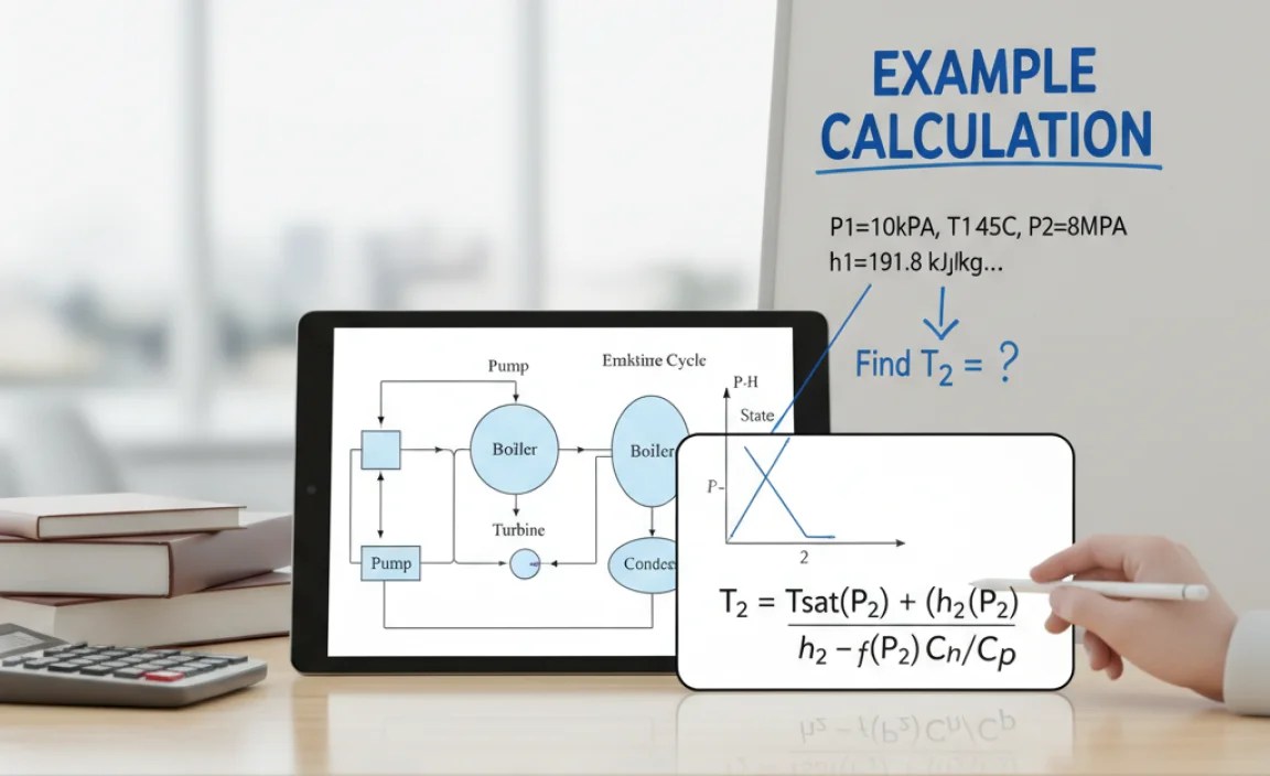
Let’s go through an example to illustrate these steps:

Given:

• Inlet Pressure (P1) = 10 kPa
• Inlet Temperature (T1) = 45°C
• Outlet Pressure (P2) = 10 MPa (10,000 kPa)
• Pump Efficiency (ηp) = 80% (0.8)

Step 1: Determine Inlet Conditions

From steam tables at P1 = 10 kPa and T1 = 45°C, we find:

• Specific Volume (v1) ≈ 0.00101 m³/kg
• Enthalpy (h1) ≈ 188.45 kJ/kg

Step 2: Calculate Isentropic Work Done

Wp,isentropic = v1 * (P2 – P1) = 0.00101 m³/kg * (10,000 kPa – 10 kPa) = 10.09 kJ/kg

Step 3: Calculate Actual Work Done

Wp,actual = Wp,isentropic / ηp = 10.09 kJ/kg / 0.8 = 12.6125 kJ/kg

Step 4: Determine Outlet Enthalpy

h2,actual = h1 + Wp,actual = 188.45 kJ/kg + 12.6125 kJ/kg = 201.0625 kJ/kg

Step 5: Find Outlet Temperature

Using steam tables or software at P2 = 10 MPa and h2,actual = 201.0625 kJ/kg, we find that the temperature T2 is approximately 45.01°C. The temperature increase is minimal, but it’s there.

This example shows that while the temperature increase is small, it’s essential to consider these calculations for accurate thermodynamic analysis.

Practical Considerations and Approximations

In many practical applications, the temperature change across the pump is often small enough to be neglected, especially when the focus is on the overall cycle performance. However, for precise calculations or in systems where even small changes can have a significant impact, it’s crucial to follow the steps outlined above.

Here are some practical considerations:

• Fluid Properties: Always use accurate thermodynamic tables or software for the specific working fluid. Different fluids will have different properties and temperature changes.
• Pump Efficiency: Don’t forget to account for pump efficiency, as real-world pumps are not perfectly isentropic.
• Approximations: In some cases, you can approximate the fluid as incompressible, simplifying the calculations. However, be aware of the limitations of this assumption.

Tools and Resources

To accurately find the temperature after a pump in a Rankine cycle, you’ll need some essential tools and resources:

• Thermodynamic Tables: These tables provide the properties of various fluids at different temperatures and pressures. Steam tables are commonly used for water. You can find these tables in most thermodynamics textbooks or online.
• Thermodynamic Software: Programs like EES (Engineering Equation Solver), CoolProp, or similar tools can calculate fluid properties and perform complex thermodynamic calculations.
• Calculators: A scientific calculator is essential for performing the necessary calculations.
• Textbooks and Online Resources: Thermodynamics textbooks and online resources like Engineering ToolBox can provide the necessary background information and formulas.

Common Mistakes to Avoid

When calculating the temperature after a pump, there are a few common mistakes to watch out for:

• Ignoring Pump Efficiency: Forgetting to account for pump efficiency will lead to inaccurate results. Always use the actual work done by the pump, not the ideal isentropic work.
• Using Incorrect Units: Ensure that all values are in consistent units (e.g., kPa for pressure, kJ/kg for enthalpy). Mixing units will result in incorrect calculations.
• Misreading Thermodynamic Tables: Be careful when reading thermodynamic tables. Ensure you’re using the correct table for the specific fluid and that you’re interpolating values accurately.
• Assuming Ideal Conditions: While assuming ideal conditions can simplify calculations, it’s essential to understand the limitations of this assumption. In real-world scenarios, factors like friction and heat loss can significantly affect the results.

Advanced Techniques and Considerations

For more advanced analysis, consider the following techniques and factors:

• Computational Fluid Dynamics (CFD): CFD simulations can provide detailed insights into the flow and temperature distribution within the pump.
• Finite Element Analysis (FEA): FEA can be used to analyze the structural integrity of the pump components under different operating conditions.
• Exergy Analysis: Exergy analysis can help identify and quantify the losses in the Rankine cycle, including those in the pump.

Rankine Cycle Components: Table of Functionality

Understanding each component’s function is vital for effective Rankine cycle analysis and optimization. The following table summarizes the functionality of each key component in the Rankine cycle.

Component	Function	Typical Operating Conditions
Pump	Increases the pressure of the working fluid.	Low pressure, low temperature (liquid)
Boiler	Heats the high-pressure fluid to create steam.	High pressure, high temperature (steam generation)
Turbine	Expands the high-pressure steam to generate power.	High pressure, high temperature (steam expansion)
Condenser	Cools the steam to convert it back into a liquid.	Low pressure, low temperature (condensation)

Typical Values in Rankine Cycle Analysis: Table of Examples

This table gives a quick overview of typical values you might encounter when analyzing a Rankine cycle. Note that these are examples, and actual values will vary based on the specific design and operating conditions of the power plant.

Parameter	Typical Value	Unit
Pump Inlet Pressure (P1)	10 – 50	kPa
Pump Outlet Pressure (P2)	5 – 20	MPa
Pump Inlet Temperature (T1)	40 – 60	°C
Turbine Inlet Temperature	400 – 600	°C
Cycle Efficiency	30 – 50	%

FAQ: Finding Temperature After a Pump in Rankine Cycle

Here are some frequently asked questions about finding the temperature after a pump in a Rankine cycle:

1. Why does the temperature increase after the pump?

The temperature increases because the pump does work on the fluid to increase its pressure. While ideally this process is isentropic (constant entropy), real-world pumps have inefficiencies that convert some of the work into heat, slightly raising the fluid’s temperature.

2. What is isentropic compression?

Isentropic compression is a thermodynamic process where the entropy of the fluid remains constant. It’s an ideal scenario that assumes no energy losses due to friction or other inefficiencies. In reality, pumps are not perfectly isentropic, but we often use this assumption for simplified calculations.

3. How do I find the enthalpy values needed for the calculations?

You can find enthalpy values using thermodynamic tables or software. Steam tables are commonly used for water. Look up the enthalpy value at the given pressure and temperature. Thermodynamic software like EES can also directly calculate enthalpy values.

4. What if the pump efficiency is not given?

If the pump efficiency is not given, you can assume an ideal isentropic process (efficiency = 100%). However, keep in mind that this will provide an idealized result. In real-world scenarios, pump efficiency typically ranges from 70% to 90%.

5. Can I ignore the temperature change in the pump?

In many practical applications, the temperature change across the pump is small enough to be neglected, especially when focusing on the overall cycle performance. However, for precise calculations or in systems where even small changes can have a significant impact, it’s crucial to calculate the temperature change.

6. What are the common units used in these calculations?

Common units include kPa or MPa for pressure, °C or K for temperature, m³/kg for specific volume, and kJ/kg for enthalpy and work. Ensure that all values are in consistent units to avoid errors in your calculations.

7. Where can I find steam tables?

Steam tables can be found in most thermodynamics textbooks, online engineering resources, and dedicated websites for thermodynamic properties. Many engineering software packages also include built-in steam tables for easy reference.

Conclusion

Finding the temperature after a pump in a Rankine cycle is a fundamental part of understanding power generation. By following these steps—determining inlet conditions, calculating work done, and using thermodynamic tables—you can accurately determine the temperature. Remember to account for pump efficiency and use consistent units to avoid errors. While the temperature change may sometimes be small enough to neglect, understanding the process ensures you can perform accurate analyses when needed. Now you’re equipped to tackle those thermodynamic challenges with confidence!

“`